Hybrid Images: Principles and Implementation
¶ 1. Introduction
A hybrid image is created by taking the high-frequency part of one image and the low-frequency part of another image, then combining them into a new image. The following is a classic textbook example:
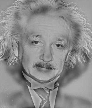
What do you see in this image?
Up close it looks like Einstein, but if you squint or view the image at a very small size, it looks like Marilyn Monroe. This happens because Einstein’s image is sharpened by a high-pass filter (emphasizing high-frequency features), while Marilyn’s image is blurred by a low-pass filter (keeping low-frequency components).
As the saying goes, “the same mountain looks different from different distances.” A hybrid image can hide more than one piece of information in a single image—and in fact, you can even hide multiple images inside one.
¶ 2. Principles
¶ 2.1 Concept
The core idea behind hybrid images is signal processing, and when we talk about signal processing we must talk about the Fourier transform.
The Fourier transform allows us to decompose a complex signal into basic components. For example:

(source from Wikipedia)
In the figure above, the original red waveform (similar to a square wave) is decomposed into multiple blue sine waves of different frequencies.
Similarly, an image is also a complex signal, and we can decompose it into a combination (superposition) of signals.
To construct a hybrid image, we take the first image, apply a Fourier transform, and keep only the high-frequency part (a high-pass). For the second image, we apply a Fourier transform and keep only the low-frequency part (a low-pass). Then we apply the inverse Fourier transform to both filtered results, and finally add the two filtered images together to obtain the hybrid image.
¶ 2.2 Math
An image can be represented as $\sum_{i, j}R_{ij}$, where $R_{ij}$ denotes the pixel value at coordinate $(i, j)$.
To apply a high-pass or low-pass, we need a filter to filter the original signal.
A filtered image $R$ is obtained by convolving the original image $F$ with a filter kernel $H$:
$$
\begin{align}
R_{ij} &= \sum_{u,v} H_{i-u, j-v} F_{u,v} \\
\mathbf R &= \mathbf H ** \mathbf F
\end{align}
$$
Here, $F$ is the 2D spectrum produced by applying a Fourier transform (FFT) to the target image and then shifting the zero frequency component to the center (FFT Shift). In this 2D spectrum, the center corresponds to low-frequency signals, while the boundary corresponds to high-frequency signals. High-frequency components represent rapid changes, edges, and corners.
The filter kernel $H$ can take many forms, but we usually use a Gaussian function $g(i,j)$, defined as:
$$g(i,j) = EXP({ -{ {(x-i)^2+(y-j)^2} \over{ 2 \sigma ^2}} })$$
Where $\sigma$ controls the scale, $(i, j)$ is the pixel coordinate, and $(x, y)$ is the center.
¶ 2.3 Filters
For why Gaussian filters are commonly used, you can refer to this discussion. In short, there are a few benefits: Gaussian filters do not produce negative values, and the filtered result tends to be closer to physical phenomena in the natural world.
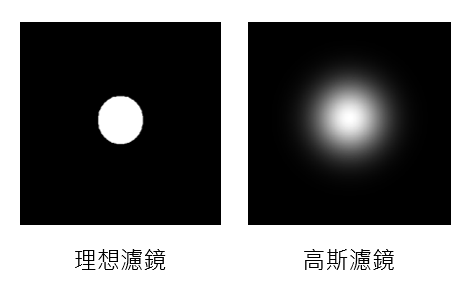
Comparing an ideal filter and a Gaussian filter: an ideal filter has a sharp boundary, while a Gaussian filter applies a smooth Gaussian function. The figure below illustrates low-pass filtering. After a Fourier transform, if we keep only the center region (white), that means the filtered image keeps only low-frequency components.
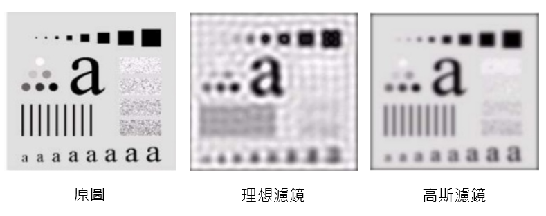
If we apply these two different low-pass filters, the low-pass effect produces blur. The results are shown below; you can see the ideal filter looks less natural.
¶ 3. Implementation
¶ 3.1 Details
First, implement the Gaussian filter:
def makeGaussianFilter(n_row, n_col, sigma, highPass=True):

    center_x = int(n_row/2) + 1 if n_row % 2 == 1 else int(n_row/2)
    center_y = int(n_col/2) + 1 if n_col % 2 == 1 else int(n_col/2)

    def gaussian(i, j):
        coefficient = math.exp(-1.0 * ((i - center_x) **
                                       2 + (j - center_y)**2) / (2 * sigma**2))
        return 1 - coefficient if highPass else coefficient

    return numpy.array(
        [[gaussian(i, j) for j in range(n_col)] for i in range(n_row)])
Then filter the image:
def filter(img, sigma, highPass):
    # 計算圖片的離散傅立葉
    shiftedDFT = fftshift(fft2(img))
    # 將 F 乘上濾鏡 H(u, v)
    filteredDFT = shiftedDFT * \
        makeGaussianFilter(
            image.shape[0], image.shape[1], sigma, highPass=isHigh)
    # 反傅立葉轉換
    res = ifft2(ifftshift(filteredDFT))

    return numpy.real(res)
shiftedDFT means we first apply a discrete Fourier transform (fft) to the image, then shift the spectrum so that frequency 0 is centered (fftshift).
Also note the return value numpy.real(res). The inverse Fourier transform produces both real and imaginary parts, often referred to as the phase spectrum and magnitude spectrum. We only need the real part, because it contains most of the image “information”; the imaginary part contains very little, and you will find the imaginary parts of different photos are often very similar. As for why—nature is just like that (a fact of nature).
Finally, we combine the high-pass and low-pass results:
def hybrid_img(high_img, low_img, sigma_h, sigma_l):
    res = filter(high_img, sigma_h, isHigh=True) + \
        filter(low_img, sigma_l, isHigh=False)
    return res
¶ 3.2 Full Code
import numpy
from numpy.fft import fft2, ifft2, fftshift, ifftshift
import math
import imageio
import matplotlib.pyplot as plt
from skimage.transform import resize


def makeGaussianFilter(n_row, n_col, sigma, highPass=True):

    center_x = int(n_row/2) + 1 if n_row % 2 == 1 else int(n_row/2)
    center_y = int(n_col/2) + 1 if n_col % 2 == 1 else int(n_col/2)

    def gaussian(i, j):
        coefficient = math.exp(-1.0 * ((i - center_x) **
                                       2 + (j - center_y)**2) / (2 * sigma**2))
        return 1 - coefficient if highPass else coefficient

    return numpy.array([[gaussian(i, j) for j in range(n_col)] for i in range(n_row)])


def filter(image, sigma, isHigh):
    shiftedDFT = fftshift(fft2(image))
    filteredDFT = shiftedDFT * \
        makeGaussianFilter(
            image.shape[0], image.shape[1], sigma, highPass=isHigh)
    res = ifft2(ifftshift(filteredDFT))

    return numpy.real(res)


def hybrid_img(high_img, low_img, sigma_h, sigma_l):
    res = filter(high_img, sigma_h, isHigh=True) + \
        filter(low_img, sigma_l, isHigh=False)
    return res


img1 = imageio.imread("IMG_PATH", as_gray=True)
img2 = imageio.imread("IMG_PATH", as_gray=True)
resize(img2, (img1.shape[0], img1.shape[1])) # 兩張圖要一樣大

plt.show(plt.imshow(hybrid_img(img1, img2, 10, 10), cmap='gray'))
Here we convert the images to grayscale (single channel), but the same idea should extend to color images (with R, G, B channels). However, when I tried to process each channel separately and then merge them back, it ended in disaster. So I’ll leave the color version as an exercise for the reader—if you succeed, feel free to share with me.
¶ 4. Results
¶ 4.1 Gaussian Low-pass and High-pass Filtering
Below are results of applying high-pass and low-pass filters to the same image using different values of $\sigma$:
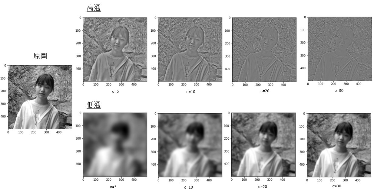
For the high-pass, a larger $\sigma$ means the “hole” carved out in the center of the spectrum becomes larger, so only the higher-frequency components near the boundary remain. As a result, you mainly see edges and contours.
For the low-pass, a smaller $\sigma$ means the preserved circle around the spectrum center becomes smaller, so more detail is lost and the result becomes blurrier.
¶ 4.2 Hybrid Images
Below are results of stacking two images after applying high-pass and low-pass filters with different $\sigma$ values:
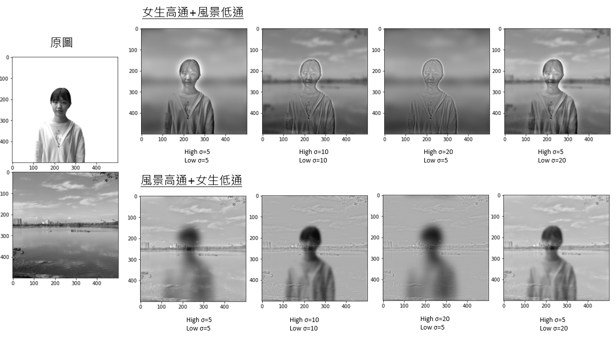
You can see that different parameter settings produce different visual effects.
¶ Conclusion
Hybrid images are made by applying a high-pass filter to one image and a low-pass filter to another, then combining them. With this technique, you can overlay two different photos according to the features you want. By adjusting $\sigma$ in the Gaussian filters, you can create hybrid images with different effects.
One practical use is steganographic watermarking: you can quietly embed a watermark by adding a very low-frequency watermark pattern into the original image. People can hardly notice it, but once you analyze it with low-pass filtering, you can discover that the source is yours.
Aha! Got caught stealing images, huh!