Rigid Body Simulation: Collision Detection, Impulses, Joint Constraints, and Numerical Methods
¶ 1. Introduction
Physics simulation is common in computer animation and games. Typical simulations include particle systems, fluid simulation, and rigid body dynamics. This post introduces collision detection, impulses and momentum transfer, joint constraints, and numerical methods in rigid body simulation.
We will cover three collision types: AABB (axis-aligned bounding boxes) vs. AABB, AABB vs. circles, and circles vs. circles. We will also describe momentum transfer and impulse resolution for rigid body collisions with friction. For constraints, we will discuss spring forces, damping forces, and fixed-length distance joints. Finally, for numerical methods we will cover Euler’s method and the Runge–Kutta method for ODEs.
¶ 2. Principles and Implementation
¶ 2.1 Collision Detection
Collision detection determines whether two objects overlap and, if they do, computes the unit normal vector (Unit Normal Vector), penetration depth (Penetration), and a boolean is-colliding flag. During simulation, each iteration checks whether a collision occurs to decide whether to resolve impulses. If a collision occurs, we use the unit normal to compute the bounce direction, and we use the unit normal and penetration depth to perform positional correction (because in theory objects should not overlap).
¶ 2.1.1 AABB vs. AABB
An AABB is axis-aligned, meaning we do not consider rotation (tilt).
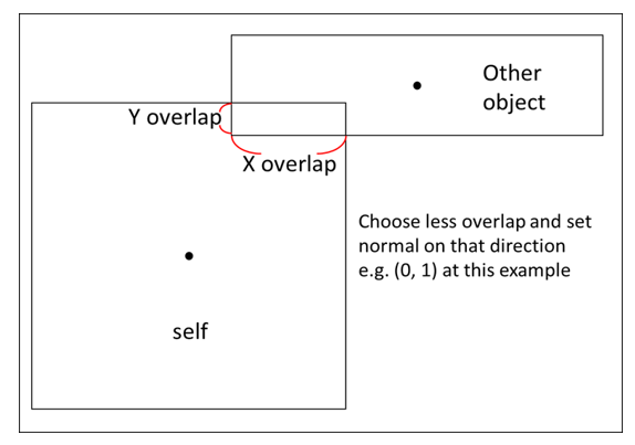
The figure below shows what it looks like when one AABB penetrates another. Based on basic physics intuition, if a square object (the “Other object” in the figure) collides horizontally or vertically, the reaction force will also be horizontal or vertical.
We define the penetration depth as the smaller overlap between the x-overlap and y-overlap. The reaction force direction is aligned with the axis of the smaller overlap.
In the example below, the normal force points along the y-overlap direction; dividing by the magnitude gives the unit normal vector.
Let the two AABBs be $A$ and $B$, and define $B$’s rebound direction as positive:
$$ penestration = min(\text {x overlap}, \text{y overlap})$$
$$ \mathbf {Normal}_{BA} =
\begin{cases}
(1, 0) &\text{if min is x overlap} \\
(0, 1) &\text{if min is x overlap}
\end{cases}
$$
To determine whether they overlap, check that all of the following are true:
$$
\begin{cases}
A.{xmax} > B.{xmin} \\
B.{xmax} > A.{xmin}\\
A.{ymax} > B.{ymin} \\
B.{ymax} > A.{ymin}
\end{cases}
$$
Pseudocode:
Note: in the pseudocode below,
float2refers tovec<float,2>.
typedef linalg::aliases::float2 float2;

float2 normal(0.0f, 0.0f);
float penetration = 0.0f;
bool is_hit = false;

if (A_x_max > B_x_min && B_x_max > A_x_min &&
    B_y_max > B_y_min && B_y_max > B_y_min)
{
    is_hit = true;
}

if (is_hit)
{
    auto overlap_x = min(A_x_max - B_x_min, B_x_max - A_x_min);
    auto overlap_y = min(B_y_max - B_y_min, B_y_max - B_y_min);

    penetration = min(overlap_x, overlap_y);

    if (penetration == overlap_x)
    {
        normal.x = B->pos.x - A->pos.x > 0 ? 1.0 : -1.0;
    }
    else
    {
        normal.y = B->pos.y - A->pos.y > 0 ? 1.0 : -1.0;
    }
}
¶ 2.1.2 Circle vs. Circle
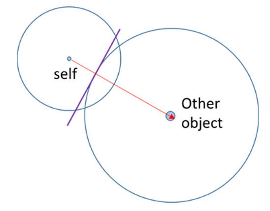
The diagram below illustrates circle–circle collision. After collision, the normal direction is along the line between the two circle centers. The penetration depth is easy to compute: the sum of the radii minus the distance between centers.
Let the radii be $R_A$ and $R_B$, the centers be $C_A$ and $C_B$, and define $\mathbf {Normal}_{BA}$ (the rebound direction of circle $B$) as positive:
$$ penestration = R_A + R_B - Distance(C_A, C_B)$$
$$ \mathbf {Normal}{BA} = \mathbf C{BA}/ Distance(C_A, C_B) $$
Pseudocode:
float2 normal(0.0f, 0.0f);
float penetration = 0.0f;
bool is_hit = false;

auto pos1 = A->pos;
auto r1 = A->radius;
auto pos2 = B->pos;
auto r2 = B->radius;

float dis = sqrt(
    (pos2.x - pos1.x) * (pos2.x - pos1.x) +
    (pos2.y - pos1.y) * (pos2.y - pos1.y));
penetration = r1 + r2 - dis;

if(penetration > 0) {
    is_hit = true;
}

normal = float2((pos2.x - pos1.x) / dis, (pos2.y - pos1.y) / dis);
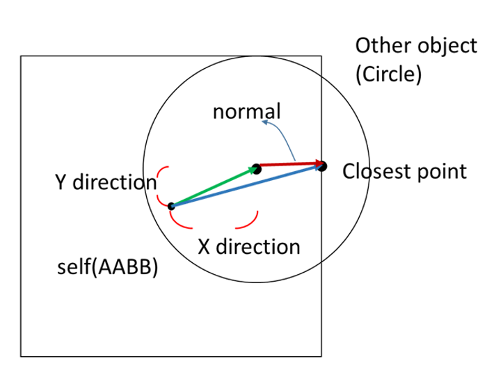
¶ 2.1.3 AABB vs. Circle
AABB–circle collision is a bit more complex. When computing the penetration depth and unit normal vector, there are two cases: (1) after collision, the circle center is outside the AABB, and (2) the circle center is inside the AABB. The computation differs slightly between the two.
¶ 2.1.3.1 Circle center outside the AABB
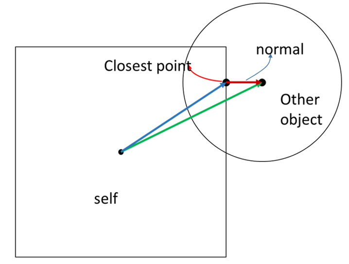
First, we find the closest point on the AABB to the circle center (Closest Point). Then we compute the vector from that closest point to the AABB center (blue) and the vector from the circle center to the AABB center (green). The normal vector is the green vector minus the blue vector.
Let the AABB be $A$, the circle be $B$, and the closest point be $P$:
$$ \mathbf N_{BA} = \mathbf V_{B_{center}A_{center}} - \mathbf V_{PA_{center}}$$
$$ penestration = B_{radius} - Distance(B_{center}, P)$$
Pseudocode:
float2 normal(0.0f, 0.0f);
float penetration = 0.0f;
bool is_hit = false;

auto ab_pos = A->pos; // AABB center
auto ab_ext = A->extent / 2;
auto x_max = ab_pos.x + ab_ext.x;
auto x_min = ab_pos.x - ab_ext.x;
auto y_max = ab_pos.y + ab_ext.y;
auto y_min = ab_pos.y - ab_ext.y;

auto c_pos = B->pos; // circle center

float2 closest_p(0, 0);

// outside
if (c_pos.x > x_max && c_pos.x < x_min &&
      c_pos.y > y_max && c_pos.y < y_min)
{
    closest_p.x = clamp(c_pos.x, x_min, x_max);
    closest_p.y = clamp(c_pos.y, y_min, y_max);

    float dis = sqrt(
        (c_pos.x - closest_p.x) * (c_pos.x - closest_p.x) +
        (closest_p.y - c_pos.y) * (closest_p.y - c_pos.y));

    penetration = B->radius - dis;

    if (penetration > 0)
    {
        is_hit = true;
        normal.x = (c_pos.x - closest_p.x) / dis;
        normal.y = (c_pos.y - closest_p.y) / dis;
    }
}
¶ 2.1.3.2 圓心在 AABB 之內
The vector definitions are the same as in the “circle center outside the AABB” case, except that the normal vector becomes the blue vector minus the green vector.
However, with an AABB we know the normal must be horizontal or vertical. So we can directly determine which side of the AABB is closest to the circle center. In the figure below, the circle center is closest to the right side of the AABB, so the closest point’s x coordinate is the AABB’s right boundary, and its y coordinate matches the circle center’s y.
$$ \mathbf N_{BA} = \mathbf V_{PA_{center}} - \mathbf V_{B_{center}A_{center}} $$
$$ penestration = B_{radius} + Distance(B_{center}, P)$$
Pseudocode (continuing from 2.1.3.2):
// inside
else
{
    auto x_right = x_max - c_pos.x;
    auto x_left = c_pos.x - x_min;
    auto y_up = y_max - c_pos.y;
    auto y_down = c_pos.y - y_min;

    auto smallest = MIN(x_right, x_left, y_up, y_down)

    if (smallest == x_right)
    {
        closest_p.x = x_max;
        closest_p.y = c_pos.y;
    }
    else if (smallest == x_left)
    {
        closest_p.x = x_min;
        closest_p.y = c_pos.y;
    }
    else if (smallest == y_down)
    {
        closest_p.x = c_pos.x;
        closest_p.y = y_min;
    }
    else
    {

        closest_p.x = c_pos.x;
        closest_p.y = y_max;
    }

    float dis = sqrt(
        (c_pos.x - closest_p.x) * (c_pos.x - closest_p.x) +
        (closest_p.y - c_pos.y) * (closest_p.y - c_pos.y));

    penetration = circle->radius + smallest;

    is_hit = true;
    normal.x = (closest_p.x - c_pos.x) / dis;
    normal.y = (closest_p.y - c_pos.y) / dis;
}
¶ 2.1.4 Positional Correction
Sometimes two objects can get “stuck” together, and we need to intervene. This situation is fairly common; here is an example.
When a small object $B$ slowly collides with object $A$, because we simulate in discrete time steps, $B$ may “sink into” $A$ before we detect the collision. Although $B$ should bounce, due to energy loss and friction, the portion of $B$ embedded in $A$ may not fully separate before $B$ comes to rest—so the two objects appear stuck together.
Another case is when an object is spawned at a position that is already occupied; they start overlapped and get stuck immediately. In these cases, we need to force them apart.
The fix is straightforward. During collision detection, we already computed the penetration depth and normal vector. So we apply a corrective displacement along the normal direction, weighted by the objects’ masses. This correction may not fully resolve overlap in one step, but because it is applied repeatedly, the objects will gradually separate until they are no longer stuck.
void correct_position(A, B)
{
  const float percent = 0.2 // typically 20% to 80% at 60 fps
  const float slop = 0.01 // only correct if penetration exceeds this, to avoid jitter; usually 0.01 to 0.1
  float2 correction = max(penetration - slop, 0.0f) / (A.inv_mass + B.inv_mass)) * percent * normal
  A.position -= A.inv_mass * correction
  B.position += B.inv_mass * correction
}
¶ 2.2 Momentum, Impulse, and Friction
In rigid body collisions, momentum is transferred between bodies, and friction also affects the outcome. During simulation, we first run collision detection. Once we confirm a collision, we resolve its effects on the bodies by applying impulses and accounting for friction.
¶ 2.2.1 Impulse Resolution
Following the “Impulse-based reaction model” section on Wikipedia’s Collision response, we can derive the impulse term for a two-body collision. I won’t repeat the full derivation here; the final result is the impulse magnitude $J_r$:
$$
\mathbf J_r = \frac{-(1 + e)((\mathbf V^B - \mathbf V^A) \cdot\mathbf n)}{\frac{1}{mass^A} + \frac{1}{mass^B}}
$$
We then apply the impulse to update the bodies’ velocities.
Pseudocode:
void Resolve(body0, body1) {
    if (isHit)
    {
        auto rel = body1->velocity - body0->velocity;
        auto vel_n = dot(rel, normal);

        // seperate
        if (vel_n > 0)
        {
            return;
        }

        // restitution
        float e = min(body0->restitution, body1->restitution);

        // impluse
        float jr = -(1 + e) * vel_n;
        jr /= body0->inv_mass + body1->inv_mass;
        auto impulse = jr * normal;

        // Apply impulse
        body0->SetVelocity(body0->velocity - body0->inv_mass * impulse);
        body1->SetVelocity(body1->velocity + body1->inv_mass * impulse);

	        /*
	            Handle friction here
	        */
    }
}
One small detail: in physics simulation we frequently use the reciprocal of mass, so it’s common to store inv_mass in the body to reduce division overhead.
¶ 2.2.2 Friction
The $J_r$ we computed can be decomposed into a normal impulse $J_n$ and a tangential impulse $J_t$. Only the tangential component produces a friction impulse.
First compute the tangential component of the relative velocity:
$$
\mathbf V^R = \mathbf V^{B}-\mathbf V^{A} \
\mathbf V^R_{tangent} =\mathbf V^R - (\mathbf V^R \cdot \mathbf n) *\mathbf n
$$
Then the tangential impulse magnitude is:
$$
\mathbf Jt = \mathbf V^R \cdot {\mathbf V^R_{tangent}\over \Vert\mathbf V^R_{tangent}\Vert}
$$
Pseudocode (continuing from the impulse resolution above):
// friction impulse

rel = body1->velocity - body0->velocity;
auto rel_normal = dot(rel, normal) * normal;
float2 rel_tan = rel - rel_normal;
float len = sqrt(rel_tan.x * rel_tan.x + rel_tan.y * rel_tan.y);

float2 tan(0, 0);
// avoid division by zero
if (len > 0.00001) {
    tan /= len;
}

auto jt = -dot(rel, tan);
jt /= body0->inv_mass + body1->inv_mass;

float2 friction_impulse(0.0f, 0.0f);
float mu = sqrt(
    pow(body0->StaticFriction, 2) + pow(body1->StaticFriction, 2));

// static friction
if (abs(jt) < jr * mu)
{
    friction_impulse = jt * tan;
}
// dynamic friction
else
{
    mu = sqrt(
        pow(body0->DynamicFriction, 2) + pow(body1->DynamicFriction, 2));
    friction_impulse = -jr * tan * mu;
}

// apply the velocity change caused by friction impulse
body0->SetVelocity(body0->velocity - body0->inv_mass * friction_impulse);
body1->SetVelocity(body1->velocity + body1->inv_mass * friction_impulse);
¶ 2.3 Joint Constraints
To simulate objects like springs or ropes, we can treat a continuous object as a chain of discrete units. During simulation, we connect many units and impose constraints on each connection. By computing the forces on each unit and combining them, we obtain the final motion of the continuous object.
¶ 2.3.1 Spring Force
When a spring is stretched or compressed, it produces a spring force. The force magnitude is proportional to the extension multiplied by the spring constant $K_S$.
The spring force between two particles $A$ and $B$ is defined as:
$$
\begin{align}
\mathbf F_a &= -K_s(\vert \mathbf x_a - \mathbf x_b \vert - length)\mathbf L&, K_s > 0 \\
&= -K_s(\vert \mathbf x_a - \mathbf x_b \vert - length){\mathbf x_a - \mathbf x_b \over{\vert \mathbf x_a - \mathbf x_b \vert}}&, K_s > 0
\end{align}
$$
Pseudocode:
auto pos_vec = body0->pos - body1->pos;
auto dis = sqrt(pow(pos_vec.x, 2) + pow(pos_vec.y, 2));

float2 f0(0.0f, 0.0f);
float2 f1(0.0f, 0.0f);

// avoid division by zero
if (dis > 0.00001)
{
    f0 = -ks * (dis - length) * pos_vec / dis;
    f1 = ks * (dis - length) * pos_vec / dis;
}

body0->force += f0
boddy1->force += f1
¶ 2.3.2 Damper Force
Similar to spring force, a damper force is a resistive force that depends on the relative velocity. The larger the velocity difference between two particles, the larger the damping force that prevents them from continuing to separate.
The damper force between two particles $A$ and $B$ is defined as follows, where $K_d$ is the damping coefficient:
$$
\begin{align}
\mathbf F_a &= -K_s((\mathbf v_a - \mathbf v_b ) \cdot \mathbf L)\mathbf L&, K_d > 0 \\
&= -K_s{(\mathbf v_a - \mathbf v_b)\cdot(\mathbf x_a - \mathbf x_b) \over{\vert \mathbf x_a - \mathbf x_b \vert}}{\mathbf x_a - \mathbf x_b \over{\vert \mathbf x_a - \mathbf x_b \vert}}&, K_s > 0
\end{align}
$$
Pseudocode:
auto pos_vec = body0->pos - body1->pos;
auto dis = sqrt(pow(pos_vec.x, 2) + pow(pos_vec.y, 2));
auto v_vec = body0->velocity - body1->velocity;

float2 f0(0.0f, 0.0f);
float2 f1(0.0f, 0.0f);
if (dis > 0.00001)
{
    f0 = -kd * (dis - lenght) * pos_vec / dis;
    f1 = kd * (dis - length) * pos_vec / dis;
}

body0->force += f0
boddy1->force += f1
¶ 2.3.3 Distance Joint (Fixed Length)
When simulating a chain, each segment has a length constraint. Two connected units cannot exceed the maximum length. When they are about to exceed it, a reaction force must counteract the tendency to stretch further.
Pseudocode:
auto pos_vec = body0->pos - body1->pos;
auto dis = sqrt(pow(pos_vec.x, 2) + pow(pos_vec.y, 2));
auto rel_dis = dis - length;

// if it exceeds the length limit
if (rel_dis > 0)
{
    // positional correction
    float2 unit_axis = pos_vec / dis;
    body1->pos = body0->pos + unit_axis * length;

    auto rel_vel = dot((body1->velocity - body0->velocity, unit_axis);
    auto remove = rel_vel + rel_dis / deltaTime;
    auto impulse = remove / (body0->inv_mass + body1->inv_mass);
    auto impulse_vec = unit_axis * impulse;
    auto force = impulse_vec / deltaTime;

    body0->force -= force;
    boddy1->force += force;
}
¶ 2.4 Numerical Methods
In physical motion, many processes can be expressed as differential equations. In simulation, we compute numerical solutions to these equations by accumulating small steps—i.e., numerically integrating. For example, displacement is the time integral of velocity.
There are many numerical methods. The physics used in this post can be modeled as first-order ordinary differential equations (ODEs), so we will introduce Euler’s method and the 4th-order Runge–Kutta method (RK4) for solving ODEs.
¶ 2.4.1 Euler Method
I won’t cover the math derivation of Euler’s method here; see Wikipedia’s Euler Method.
Below is example pseudocode for using Euler’s method to simulate motion under forces:
void timeStep(body) {
    body->velocity += body->force * delta_time / body->mass; // Ft = mv
    body->pos += delta_time * vel;
}
In this example, we integrate over time. From $F \Delta t=m \Delta v$, at each time step we obtain the change in velocity, and then use the updated velocity to compute the change in position.
¶ 2.4.2 Runge–Kutta Method
For the mathematical derivation of Runge–Kutta, see Wikipedia’s Runge–Kutta methods.
Below is example pseudocode for using Runge–Kutta to simulate motion under gravitational acceleration:
void timeStep(body) {
    auto f = [=](StateStep &step, float2 vel, float t) {
        vel += gravity * t;
        step.velocity = vel;
    };

    StateStep F0, F1, F2, F3, F4;
    F0.velocity = float2(0,0);
    f(F1, F0.velocity, 0);
    f(F2, F1.velocity / 2, deltaTime / 2);
    f(F3, F2.velocity / 2, deltaTime / 2);
    f(F4, F3.velocity, deltaTime);

    auto v0 = body->vel + body->force * deltaTime / body->mass;
    body->vel =  v0 + (F1.velocity + 2 * F2.velocity + 2 * F3.velocity + F4.velocity) / 6;
    body->pos += body->vel * deltaTime;
}
¶ 3. Results and Discussion
¶ 3.1 Extending Collision Detection
In this post, we only discussed collisions involving AABBs and circles. Obviously, real-world shapes are not limited to AABBs and circles. Even for “boxes”, once rotation is involved, the computation changes significantly. For collision detection of rotated polygons, you can refer to the Separating Axis Theorem (SAT).
Also, the real world is 3D. Handling collision detection for 3D objects goes beyond SAT in 2D and is a more complex topic.
¶ 3.2 Torque and Moment of Inertia
In this post, we ignored torque and moment of inertia. In reality, objects also experience angular impulses during impacts. Why didn’t we cover rotation here? Because once rotation is involved, a square is no longer an AABB, and you need SAT to determine collisions. Due to space constraints, readers who are interested can refer to “How to Create a Custom 2D Physics Engine: Oriented Rigid Bodies”, first understand SAT, and then implement rotation and moment of inertia based on physics principles.
¶ 3.3 Euler vs. Runge–Kutta
Euler’s method is a first-order method: it uses the current rate of change to compute the next step. It is simple and easy to implement, but because each step adds only the rate at that step, the simulation can become inaccurate if the step size (Delta) is too large. To get accurate results, the step size must be small, which makes the computation expensive.
Runge–Kutta can be generalized to an $n$-th order RK method, but in practice we often use 4th order (RK4) to balance accuracy and speed. RK4 takes four intermediate estimates and forms a weighted average. It performs well for differential equations up to order four. Because it is less sensitive to step size (Delta), you can often use a larger step size to compute faster while still obtaining a more accurate numerical solution.
¶ 4. Conclusion
With numerical simulation, we can bring real-world physics into computer animation and games. This post explored collision detection, impulses and momentum transfer, joint constraints, and numerical methods in rigid body motion. Rigid body dynamics is one of the most common applications—mobile games like Angry Birds are a classic example, where you need to compute trajectories and handle collisions and impulse transfer when birds hit wood or stone. Using the methods described here, you can implement a simple collision simulation. For deeper study, you can look into the differences between 2D and 3D simulation, as well as more sophisticated physical models and numerical techniques.
¶ 5. References