剛体シミュレーション:衝突判定、インパルス、ジョイント制約、数値解法
¶ 1. はじめに
コンピュータアニメーションやゲームでは、物理シミュレーションが頻繁に必要になります。よくある物理シミュレーションには、パーティクルシステム、流体シミュレーション、剛体運動などがあります。本記事では、剛体(Rigid Body)シミュレーションにおける衝突判定、インパルスによる運動量の移動、ジョイント制約、数値解法を紹介します。
衝突判定は、AABB(Axis-aligned Bounding Boxes)と AABB、AABB と円、円と円の 3 種類を扱います。また、摩擦力を考慮した剛体衝突における運動量移動とインパルス解決について説明します。制約としては、ばね力、ダンパ(減衰)力、固定長の距離ジョイントを扱います。最後に、数値解法として常微分方程式(ODE)に対するオイラー法(Euler Method)とルンゲ=クッタ法(Runge–Kutta)を取り上げます。
¶ 2. 原理と実装
¶ 2.1 衝突判定(Collision Detection)
衝突判定(collision detection)は、2 つの物体が重なっているかを判定し、衝突時の 単位法線ベクトル(Unit Normal Vector)、貫通量(Penetration)、衝突しているかどうか(is-colliding)を求めます。シミュレーションでは、各イテレーションで「衝突しているか」を確認し、衝突していればインパルス解決を行います。また、理論上は物体が重なってはいけないため、単位法線ベクトルと貫通量を使って位置補正(positional correction)も行います。
¶ 2.1.1 AABB と AABB の衝突
AABB は軸に整列した(axis-aligned)矩形であり、回転(傾き)は考慮しません。
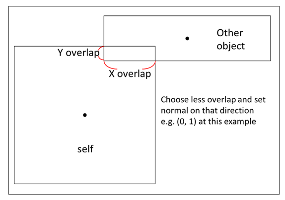
次の図は、AABB が AABB に貫通した状態を示しています。物理的な直感として、正方形の物体(図中の Other object)が水平方向または垂直方向に衝突した場合、反作用力も水平方向または垂直方向になります。
貫通量は、x 方向の重なり(Overlap)と y 方向の重なりのうち小さいほうを採用します。反作用力の向きは、この「小さい重なり」の軸方向に一致します。
次の例では、法線方向の力は y-overlap の方向になります。y-overlap の大きさで割ると単位法線ベクトルが得られます。
2 つの AABB を $A$ と $B$ とし、$B$ の反発方向を正と定義します:
$$ penestration = min(\text {x overlap}, \text{y overlap})$$
$$ \mathbf {Normal}_{BA} =
\begin{cases}
(1, 0) &\text{if min is x overlap} \\
(0, 1) &\text{if min is x overlap}
\end{cases}
$$
重なりがあるかどうかは、次の条件がすべて真であることを確認します:
$$
\begin{cases}
A.{xmax} > B.{xmin} \\
B.{xmax} > A.{xmin}\\
A.{ymax} > B.{ymin} \\
B.{ymax} > A.{ymin}
\end{cases}
$$
擬似コード:
注意:以下の擬似コードでは
float2はvec<float,2>を指します。
typedef linalg::aliases::float2 float2;

float2 normal(0.0f, 0.0f);
float penetration = 0.0f;
bool is_hit = false;

if (A_x_max > B_x_min && B_x_max > A_x_min &&
    B_y_max > B_y_min && B_y_max > B_y_min)
{
    is_hit = true;
}

if (is_hit)
{
    auto overlap_x = min(A_x_max - B_x_min, B_x_max - A_x_min);
    auto overlap_y = min(B_y_max - B_y_min, B_y_max - B_y_min);

    penetration = min(overlap_x, overlap_y);

    if (penetration == overlap_x)
    {
        normal.x = B->pos.x - A->pos.x > 0 ? 1.0 : -1.0;
    }
    else
    {
        normal.y = B->pos.y - A->pos.y > 0 ? 1.0 : -1.0;
    }
}
¶ 2.1.2 円と円の衝突
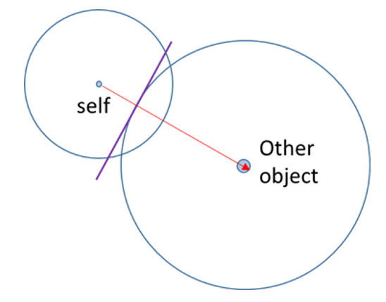
次の図は、円と円の衝突を示しています。衝突後の法線方向は 2 つの円の中心を結ぶ直線方向になります。貫通量は簡単で、半径の和から中心間距離を引いたものです。
半径を $R_A$ と $R_B$、中心を $C_A$ と $C_B$ とし、円 $B$ の反発方向である $\mathbf {Normal}_{BA}$ を正と定義します:
$$ penestration = R_A + R_B - Distance(C_A, C_B)$$
$$ \mathbf {Normal}{BA} = \mathbf C{BA}/ Distance(C_A, C_B) $$
擬似コード:
float2 normal(0.0f, 0.0f);
float penetration = 0.0f;
bool is_hit = false;

auto pos1 = A->pos;
auto r1 = A->radius;
auto pos2 = B->pos;
auto r2 = B->radius;

float dis = sqrt(
    (pos2.x - pos1.x) * (pos2.x - pos1.x) +
    (pos2.y - pos1.y) * (pos2.y - pos1.y));
penetration = r1 + r2 - dis;

if(penetration > 0) {
    is_hit = true;
}

normal = float2((pos2.x - pos1.x) / dis, (pos2.y - pos1.y) / dis);
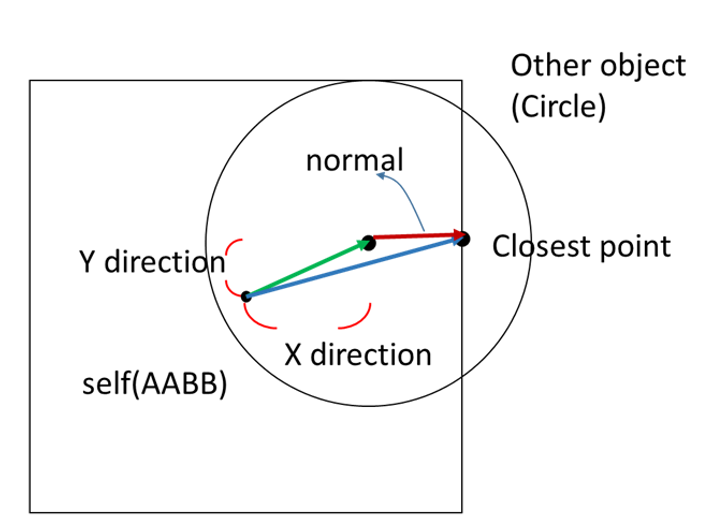
¶ 2.1.3 AABB と円の衝突
AABB と円の衝突は少し複雑です。貫通量と単位法線ベクトルを求めるとき、(1) 衝突後に円の中心が AABB の外側にある場合と、(2) 円の中心が AABB の内側にある場合の 2 パターンがあり、計算方法が少し異なります。
¶ 2.1.3.1 円の中心が AABB の外側にある場合
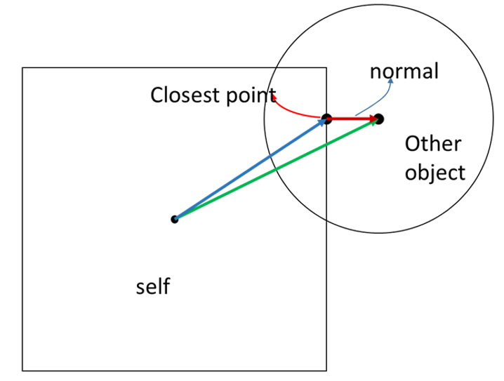
まず、円の中心に最も近い AABB 上の点(Closest Point)を求めます。次に、その最近点から AABB 中心へのベクトル(青)と、円の中心から AABB 中心へのベクトル(緑)を求めます。法線ベクトルは「緑ベクトル − 青ベクトル」になります。
AABB を $A$、円を $B$、最近点を $P$ とします:
$$ \mathbf N_{BA} = \mathbf V_{B_{center}A_{center}} - \mathbf V_{PA_{center}}$$
$$ penestration = B_{radius} - Distance(B_{center}, P)$$
擬似コード:
float2 normal(0.0f, 0.0f);
float penetration = 0.0f;
bool is_hit = false;

auto ab_pos = A->pos; // AABB center
auto ab_ext = A->extent / 2;
auto x_max = ab_pos.x + ab_ext.x;
auto x_min = ab_pos.x - ab_ext.x;
auto y_max = ab_pos.y + ab_ext.y;
auto y_min = ab_pos.y - ab_ext.y;

auto c_pos = B->pos; // circle center

float2 closest_p(0, 0);

// outside
if (c_pos.x > x_max && c_pos.x < x_min &&
      c_pos.y > y_max && c_pos.y < y_min)
{
    closest_p.x = clamp(c_pos.x, x_min, x_max);
    closest_p.y = clamp(c_pos.y, y_min, y_max);

    float dis = sqrt(
        (c_pos.x - closest_p.x) * (c_pos.x - closest_p.x) +
        (closest_p.y - c_pos.y) * (closest_p.y - c_pos.y));

    penetration = B->radius - dis;

    if (penetration > 0)
    {
        is_hit = true;
        normal.x = (c_pos.x - closest_p.x) / dis;
        normal.y = (c_pos.y - closest_p.y) / dis;
    }
}
¶ 2.1.3.2 圓心在 AABB 之內
ベクトルの定義は「円の中心が AABB の外側にある場合」と同じですが、法線ベクトルが「青ベクトル − 緑ベクトル」になります。
ただし AABB の場合、法線は水平または垂直のどちらかに限られます。そのため、円の中心が AABB のどの辺に最も近いかを直接判定できます。次の図では、円の中心が AABB の右辺に最も近いので、最近点の x 座標は AABB の右端になり、y 座標は円の中心の y と同じになります。
$$ \mathbf N_{BA} = \mathbf V_{PA_{center}} - \mathbf V_{B_{center}A_{center}} $$
$$ penestration = B_{radius} + Distance(B_{center}, P)$$
擬似コード(2.1.3.2 の続き):
// inside
else
{
    auto x_right = x_max - c_pos.x;
    auto x_left = c_pos.x - x_min;
    auto y_up = y_max - c_pos.y;
    auto y_down = c_pos.y - y_min;

    auto smallest = MIN(x_right, x_left, y_up, y_down)

    if (smallest == x_right)
    {
        closest_p.x = x_max;
        closest_p.y = c_pos.y;
    }
    else if (smallest == x_left)
    {
        closest_p.x = x_min;
        closest_p.y = c_pos.y;
    }
    else if (smallest == y_down)
    {
        closest_p.x = c_pos.x;
        closest_p.y = y_min;
    }
    else
    {

        closest_p.x = c_pos.x;
        closest_p.y = y_max;
    }

    float dis = sqrt(
        (c_pos.x - closest_p.x) * (c_pos.x - closest_p.x) +
        (closest_p.y - c_pos.y) * (closest_p.y - c_pos.y));

    penetration = circle->radius + smallest;

    is_hit = true;
    normal.x = (closest_p.x - c_pos.x) / dis;
    normal.y = (closest_p.y - c_pos.y) / dis;
}
¶ 2.1.4 位置補正
2 つの物体が「めり込んだまま固まる」ことがあり、その場合は介入して処理する必要があります。これは比較的よく起きます。例を挙げます。
小さな物体 $B$ が物体 $A$ にゆっくり衝突する場合、離散的なタイムステップでシミュレーションしているため、衝突を検出する時点ではすでに $B$ が $A$ の内部に「めり込んで」いることがあります。本来なら $B$ は反発しますが、内部エネルギーの損失や摩擦の影響で、$B$ が $A$ から完全に離れきる前に停止してしまい、結果として 2 つの物体が引っかかったように見えます。
また、生成された物体が最初から他の物体と重なった位置に出現すると、その時点で即座に「固まり」ます。こうした場合は強制的に押し出して分離させます。
処理は単純です。衝突判定の段階で貫通量と法線ベクトルを求めているので、質量(正確には逆質量)に応じて、法線方向へ補正量だけ位置をずらします。この補正は 1 回で完全に解消しないこともありますが、毎フレーム適用されるため、徐々にめり込みが解消されていきます。
void correct_position(A, B)
{
	  const float percent = 0.2 // 60fps では通常 20%〜80% 程度
	  const float slop = 0.01 // ジッタを避けるため、貫通が一定量を超えたときのみ補正する(通常 0.01〜0.1)
  float2 correction = max(penetration - slop, 0.0f) / (A.inv_mass + B.inv_mass)) * percent * normal
  A.position -= A.inv_mass * correction
  B.position += B.inv_mass * correction
}
¶ 2.2 運動量・インパルス・摩擦
剛体の衝突では、物体間で運動量が移動し、摩擦も結果に影響します。シミュレーションではまず衝突判定を行い、衝突が確認できたらインパルスを適用し、摩擦も考慮して物体の状態を更新します。
¶ 2.2.1 インパルス解決
Wikipedia の Collision response にある “Impulse-based reaction model” の説明に従うと、2 物体の衝突におけるインパルス項を導出できます。ここでは導出過程は省略し、最終的に衝突時のインパルスの大きさ $J_r$ は次のようになります:
$$
\mathbf J_r = \frac{-(1 + e)((\mathbf V^B - \mathbf V^A) \cdot\mathbf n)}{\frac{1}{mass^A} + \frac{1}{mass^B}}
$$
このインパルスを用いて、各物体の速度を更新します。
擬似コード:
void Resolve(body0, body1) {
    if (isHit)
    {
        auto rel = body1->velocity - body0->velocity;
        auto vel_n = dot(rel, normal);

        // seperate
        if (vel_n > 0)
        {
            return;
        }

        // restitution
        float e = min(body0->restitution, body1->restitution);

        // impluse
        float jr = -(1 + e) * vel_n;
        jr /= body0->inv_mass + body1->inv_mass;
        auto impulse = jr * normal;

        // Apply impulse
        body0->SetVelocity(body0->velocity - body0->inv_mass * impulse);
        body1->SetVelocity(body1->velocity + body1->inv_mass * impulse);

		        /*
		            ここで摩擦を処理する
		        */
    }
}
補足:物理シミュレーションでは質量の逆数を頻繁に使うため、除算のオーバーヘッドを減らす目的で、inv_mass(逆質量)をボディ側に保持しておくことが一般的です。
¶ 2.2.2 摩擦
先ほど求めた $J_r$ は、法線方向のインパルス $J_n$ と接線方向のインパルス $J_t$ に分解できます。摩擦インパルスが生じるのは接線方向成分のみです。
まず相対速度の接線成分を計算します:
$$
\mathbf V^R = \mathbf V^{B}-\mathbf V^{A} \
\mathbf V^R_{tangent} =\mathbf V^R - (\mathbf V^R \cdot \mathbf n) *\mathbf n
$$
接線方向インパルスの大きさは次の通りです:
$$
\mathbf Jt = \mathbf V^R \cdot {\mathbf V^R_{tangent}\over \Vert\mathbf V^R_{tangent}\Vert}
$$
擬似コード(上のインパルス解決の続き):
// 摩擦インパルス

rel = body1->velocity - body0->velocity;
auto rel_normal = dot(rel, normal) * normal;
float2 rel_tan = rel - rel_normal;
float len = sqrt(rel_tan.x * rel_tan.x + rel_tan.y * rel_tan.y);

float2 tan(0, 0);
// 0 除算を避ける
if (len > 0.00001) {
    tan /= len;
}

auto jt = -dot(rel, tan);
jt /= body0->inv_mass + body1->inv_mass;

float2 friction_impulse(0.0f, 0.0f);
float mu = sqrt(
    pow(body0->StaticFriction, 2) + pow(body1->StaticFriction, 2));

// 静摩擦
if (abs(jt) < jr * mu)
{
    friction_impulse = jt * tan;
}
// 動摩擦
else
{
    mu = sqrt(
        pow(body0->DynamicFriction, 2) + pow(body1->DynamicFriction, 2));
    friction_impulse = -jr * tan * mu;
}

// 摩擦インパルスによる速度変化を適用
body0->SetVelocity(body0->velocity - body0->inv_mass * friction_impulse);
body1->SetVelocity(body1->velocity + body1->inv_mass * friction_impulse);
¶ 2.3 ジョイント制約(Joint Constraint)
ばねやロープのような連続体をシミュレーションする場合、連続体を複数の単位要素の連結として近似できます。シミュレーションでは多数の単位要素をつなぎ、各接続に制約を課すことで、各単位要素に作用する力を計算し、それらを合成して連続体としての最終的な運動を得ます。
¶ 2.3.1 ばね力(Spring Force)
ばねが伸びたり縮んだりすると、ばね力が発生します。ばね力は伸長量にばね定数 $K_S$ を掛けたものとして定義されます。
2 つの質点 $A$ と $B$ の間のばね力は次のように定義できます:
$$
\begin{align}
\mathbf F_a &= -K_s(\vert \mathbf x_a - \mathbf x_b \vert - length)\mathbf L&, K_s > 0 \\
&= -K_s(\vert \mathbf x_a - \mathbf x_b \vert - length){\mathbf x_a - \mathbf x_b \over{\vert \mathbf x_a - \mathbf x_b \vert}}&, K_s > 0
\end{align}
$$
擬似コード:
auto pos_vec = body0->pos - body1->pos;
auto dis = sqrt(pow(pos_vec.x, 2) + pow(pos_vec.y, 2));

float2 f0(0.0f, 0.0f);
float2 f1(0.0f, 0.0f);

// 0 除算を避ける
if (dis > 0.00001)
{
    f0 = -ks * (dis - length) * pos_vec / dis;
    f1 = ks * (dis - length) * pos_vec / dis;
}

body0->force += f0
boddy1->force += f1
¶ 2.3.2 ダンパ力(Damper Force)
ばね力と同様に、ダンパ力は相対速度差に応じて発生する抵抗力です。2 つの質点の速度差が大きいほど、分離し続けるのを抑えるダンパ力も大きくなります。
2 つの質点 $A$ と $B$ の間のダンパ力は次のように定義できます($K_d$ は減衰係数):
$$
\begin{align}
\mathbf F_a &= -K_s((\mathbf v_a - \mathbf v_b ) \cdot \mathbf L)\mathbf L&, K_d > 0 \\
&= -K_s{(\mathbf v_a - \mathbf v_b)\cdot(\mathbf x_a - \mathbf x_b) \over{\vert \mathbf x_a - \mathbf x_b \vert}}{\mathbf x_a - \mathbf x_b \over{\vert \mathbf x_a - \mathbf x_b \vert}}&, K_s > 0
\end{align}
$$
擬似コード:
auto pos_vec = body0->pos - body1->pos;
auto dis = sqrt(pow(pos_vec.x, 2) + pow(pos_vec.y, 2));
auto v_vec = body0->velocity - body1->velocity;

float2 f0(0.0f, 0.0f);
float2 f1(0.0f, 0.0f);
if (dis > 0.00001)
{
    f0 = -kd * (dis - lenght) * pos_vec / dis;
    f1 = kd * (dis - length) * pos_vec / dis;
}

body0->force += f0
boddy1->force += f1
¶ 2.3.3 固定長ジョイント(Distance Joint)
鎖(チェーン)をシミュレーションする場合、各ユニットには長さ制約があります。連結された 2 つのユニット間の距離は制限を超えられず、超えそうになった場合は、これ以上伸びないように反作用力が働く必要があります。
擬似コード:
auto pos_vec = body0->pos - body1->pos;
auto dis = sqrt(pow(pos_vec.x, 2) + pow(pos_vec.y, 2));
auto rel_dis = dis - length;

// 長さ制約を超えた場合
if (rel_dis > 0)
{
    // 位置補正
    float2 unit_axis = pos_vec / dis;
    body1->pos = body0->pos + unit_axis * length;

    auto rel_vel = dot((body1->velocity - body0->velocity, unit_axis);
    auto remove = rel_vel + rel_dis / deltaTime;
    auto impulse = remove / (body0->inv_mass + body1->inv_mass);
    auto impulse_vec = unit_axis * impulse;
    auto force = impulse_vec / deltaTime;

    body0->force -= force;
    boddy1->force += force;
}
¶ 2.4 数値解法(Numerical Methods)
物理運動は、多くの場合、微分方程式として表現できます。シミュレーションでは、微分方程式の数値解を求めるために、小さなステップを積み上げる形で数値積分します。たとえば位置の変化は、速度を時間積分したものです。
数値解法には多くの種類があります。本記事で扱う物理は 1 階の常微分方程式(ODE)として表現できるため、ODE の数値解法としてオイラー法と 4 次のルンゲ=クッタ法(RK4)を紹介します。
¶ 2.4.1 オイラー法(Euler Method)
オイラー法の数学的導出はここでは扱いません。Wikipedia の Euler Method を参照してください。
以下は、力を受ける物体の運動をオイラー法で扱う擬似コード例です:
void timeStep(body) {
    body->velocity += body->force * delta_time / body->mass; // Ft = mv
    body->pos += delta_time * vel;
}
この例では時間方向に積分します。$F \Delta t=m \Delta v$ より、各タイムステップで速度の変化量を得て、更新後の速度から位置の変化量を計算します。
¶ 2.4.2 ルンゲ=クッタ法(Runge–Kutta Method)
ルンゲ=クッタ法の数学的導出は、Wikipedia の Runge–Kutta methods を参照してください。
以下は、重力加速度を受ける物体の運動をルンゲ=クッタ法で扱う擬似コード例です:
void timeStep(body) {
    auto f = [=](StateStep &step, float2 vel, float t) {
        vel += gravity * t;
        step.velocity = vel;
    };

    StateStep F0, F1, F2, F3, F4;
    F0.velocity = float2(0,0);
    f(F1, F0.velocity, 0);
    f(F2, F1.velocity / 2, deltaTime / 2);
    f(F3, F2.velocity / 2, deltaTime / 2);
    f(F4, F3.velocity, deltaTime);

    auto v0 = body->vel + body->force * deltaTime / body->mass;
    body->vel =  v0 + (F1.velocity + 2 * F2.velocity + 2 * F3.velocity + F4.velocity) / 6;
    body->pos += body->vel * deltaTime;
}
¶ 3. 結果と考察
¶ 3.1 衝突判定の拡張
本記事では AABB と円の衝突だけを扱いましたが、現実世界の形状は当然それだけではありません。さらに「箱」でも、回転が入るだけで計算方法は大きく変わります。回転した多角形の衝突判定については、Separating Axis Theorem(SAT)を参照してください。
また、現実世界は 3D です。3D 物体の衝突判定は 2D の SAT だけでは扱えず、より複雑な分野になります。
¶ 3.2 トルクと慣性モーメント
本記事ではトルクと慣性モーメントを無視しました。実際の物体は衝突時に回転方向のインパルスも受けます。なぜ回転を扱わなかったかというと、回転が絡むと正方形は AABB ではなくなり、衝突判定に SAT の説明が必要になるためです。紙幅の都合上、興味のある方は「How to Create a Custom 2D Physics Engine: Oriented Rigid Bodies」を参照し、まず SAT を理解した上で、物理学に基づいて回転と慣性モーメントを実装してください。
¶ 3.3 オイラー法とルンゲ=クッタ法の比較
オイラー法は 1 次の方法で、変化率(rate)から次のステップを求めます。原理が単純で実装しやすい一方、各ステップでその時点の変化率だけを加算するため、ステップ幅(Delta)が大きいとシミュレーションが歪みやすいです。精度を上げるにはステップ幅を小さくする必要があり、その分計算コストが増えます。
ルンゲ=クッタ法は $n$ 次の RK 法として一般化できますが、精度と速度のバランスのために 4 次(RK4)がよく使われます。RK4 は 4 通りの中間推定を取り、加重平均して更新します。4 次以内の微分方程式に対して良い性質を持ち、ステップ幅(Delta)への感度が比較的低いため、ステップ幅を大きめにしても比較的良い数値解が得られることがあります。
¶ 4. まとめ
数値シミュレーションにより、現実世界の物理をコンピュータアニメーションやゲームへ持ち込めます。本記事では、剛体運動における衝突判定、インパルス(運動量の移動)、ジョイント制約、数値解法を扱いました。剛体運動は最も一般的な応用の一つで、たとえば Angry Birds のようなゲームでは、鳥が飛んだ軌跡の計算や、木・石に衝突したときの衝突判定とインパルスによる運動量移動が必要になります。本記事の方法を使えば、簡単な衝突シミュレーションを実装できます。より深く学ぶには、2D と 3D シミュレーションの違いや、より精密な物理モデル、数値計算法などを調べるとよいでしょう。
¶ 5. 参考資料