Neutrino's Blog

¶ 1. 簡介

電腦動畫或電腦遊戲中常常都會需要做物理模擬，常見的物理模擬有粒子系統、流體模擬、剛體運動等等。本文主要介紹剛體 (Rigid Body) 運動中的碰撞偵測、動量衝量、連結限制 (Joint Constraint) 以及數值方法。

本文會介紹碰撞偵測包含 AABB (Axis-aligned Bounding Boxes) 與 AABB、AABB 和圓形以及圓形和圓形這三種碰撞型態。描述剛體碰撞時，動量與衝量在考慮有摩擦力的情況下的轉移。也會討論包含彈簧力、阻力和固定長度這三種於剛體系統的連結限制。最後數值法討論 OED 的尤拉法 (Euler Method) 和 Runge Kutta 法。

¶ 2. 原理和實現

¶ 2.1 碰撞偵測

碰撞偵測的判斷方式是看兩者有沒有重疊部分，求出碰撞時的單位正向向量 (Unit Normal Vector)、穿透量 (Penetration)、是否碰撞。模擬過程中，每次迭代都檢查是否碰撞決定是否要做動量衝量計算，如果有碰撞了，就會用到單位正向向量來算反彈方向，以及單位正向向量和穿透量來做位置修正，因為理論上物體不會有重疊。

¶ 2.1.1 AABB 與 AABB 碰撞

AABB 定義是沿著軸擺 (Axis-aligned)，也就是不考慮如果歪斜的形況。

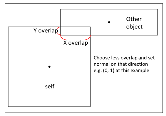
下圖是 AABB (Axis-aligned Bounding Boxes) 與 AABB 碰撞穿透後的樣子，基於我們對物理的概念，如果一個方形物體 (圖中的 Other object) 以水平或垂直方向碰撞，那反作用力也會是水平或垂直。

我們定義穿透量取 X 重疊 (Overlap) 和 Y 重疊較短邊，並且反作用力的向量方向會和最較短重疊的方向一致。

以下圖為例，正向力會沿著 Y overlap 方向，除以 Y overlap 量值之後得到單位正向向量。

定義兩 AABB 為 A 和 B，B 反彈方向為正：

$$ penestration = min(\text {x overlap}, \text{y overlap})$$
$$ \mathbf {Normal}_{BA} =
\begin{cases}
(1, 0) &\text{if min is x overlap} \\
(0, 1) &\text{if min is x overlap}
\end{cases}
$$

此外如果如果想知道有沒有重疊的話，只要檢查下列是否都為真：

$$
\begin{cases}
A.{xmax} > B.{xmin} \\
B.{xmax} > A.{xmin}\\
A.{ymax} > B.{ymin} \\
B.{ymax} > A.{ymin}
\end{cases}
$$

虛擬碼：

注意到之後虛擬碼中的 float2 都是 vec<float,2>

typedef linalg::aliases::float2 float2;

float2 normal(0.0f, 0.0f);
float penetration = 0.0f;
bool is_hit = false;

if (A_x_max > B_x_min && B_x_max > A_x_min &&
    B_y_max > B_y_min && B_y_max > B_y_min)
{
    is_hit = true;
}

if (is_hit)
{
    auto overlap_x = min(A_x_max - B_x_min, B_x_max - A_x_min);
    auto overlap_y = min(B_y_max - B_y_min, B_y_max - B_y_min);

    penetration = min(overlap_x, overlap_y);

    if (penetration == overlap_x)
    {
        normal.x = B->pos.x - A->pos.x > 0 ? 1.0 : -1.0;
    }
    else
    {
        normal.y = B->pos.y - A->pos.y > 0 ? 1.0 : -1.0;
    }
}

¶ 2.1.2 圓形與圓形碰撞

圓形與圓型碰撞的示意圖如下，碰撞後的正向力方向為沿著兩圓心，而穿透量也很簡單計算，亦即兩半徑相加減掉兩圓心距離。

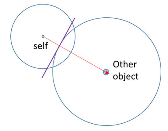
定義兩圓半徑分別是 $R_A$ 和 $R_B$，兩圓圓心分別是 $C_A$ 和 $C_B$，且定 B 圓反彈方向 $\mathbf {Normal}_{BA}$ 為正：

$$ penestration = R_A + R_B - Distance(C_A, C_B)$$
$$ \mathbf {Normal}{BA} = \mathbf C{BA}/ Distance(C_A, C_B) $$

虛擬碼：

float2 normal(0.0f, 0.0f);
float penetration = 0.0f;
bool is_hit = false;

auto pos1 = A->pos;
auto r1 = A->radius;
auto pos2 = B->pos;
auto r2 = B->radius;

float dis = sqrt(
    (pos2.x - pos1.x) * (pos2.x - pos1.x) +
    (pos2.y - pos1.y) * (pos2.y - pos1.y));
penetration = r1 + r2 - dis;

if(penetration > 0) {
    is_hit = true;
}

normal = float2((pos2.x - pos1.x) / dis, (pos2.y - pos1.y) / dis);

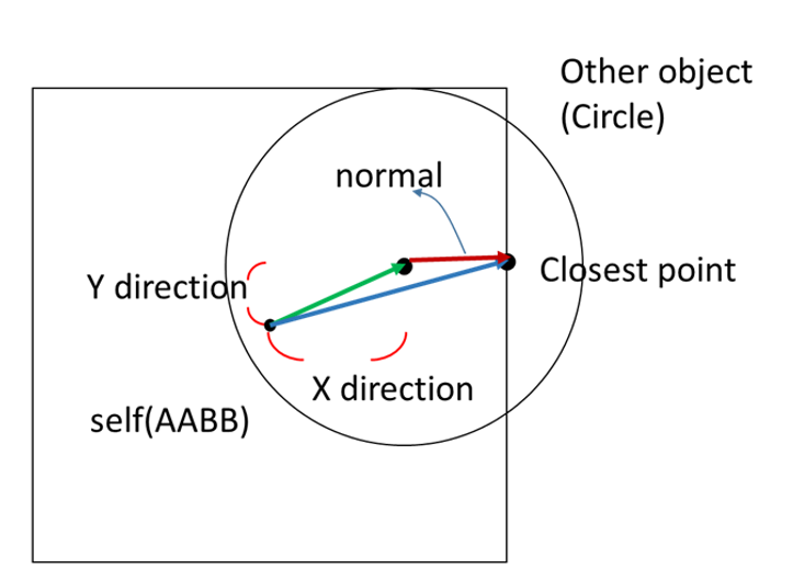
¶ 2.1.3 AABB 與圓形的碰撞

AABB 與圓形碰撞就比較複雜，在求穿透量和單位正向向量時情況分兩種，一種是碰撞後圓心在 AABB 之外，另一種是圓心在 AABB 之內，計算方法會有點差別。

¶ 2.1.3.1 圓心在 AABB 之外

首先我們要找到 AABB 離圓形圓心最近的點 (Closest Point)，並得到最近的點到 AABB 中心的向量 (藍色)，和得到圓心到 AABB 中心的向量 (綠色)
，而正向量則為綠色向量減掉藍色向量。

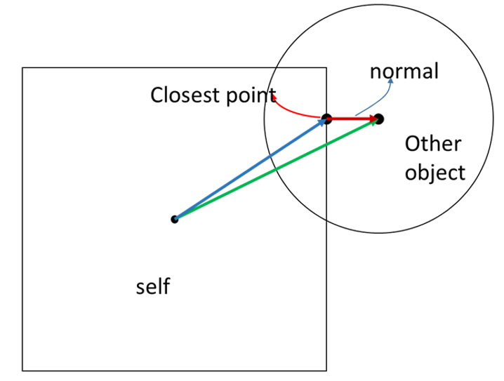
定義 AABB 為 A，圓形為 B，最近點為 P：

$$ \mathbf N_{BA} = \mathbf V_{B_{center}A_{center}} - \mathbf V_{PA_{center}}$$
$$ penestration = B_{radius} - Distance(B_{center}, P)$$

虛擬碼：

float2 normal(0.0f, 0.0f);
float penetration = 0.0f;
bool is_hit = false;

auto ab_pos = A->pos; // AABB center
auto ab_ext = A->extent / 2;
auto x_max = ab_pos.x + ab_ext.x;
auto x_min = ab_pos.x - ab_ext.x;
auto y_max = ab_pos.y + ab_ext.y;
auto y_min = ab_pos.y - ab_ext.y;

auto c_pos = B->pos; // circle center

float2 closest_p(0, 0);

// outside
if (c_pos.x > x_max && c_pos.x < x_min &&
      c_pos.y > y_max && c_pos.y < y_min)
{
    closest_p.x = clamp(c_pos.x, x_min, x_max);
    closest_p.y = clamp(c_pos.y, y_min, y_max);

    float dis = sqrt(
        (c_pos.x - closest_p.x) * (c_pos.x - closest_p.x) +
        (closest_p.y - c_pos.y) * (closest_p.y - c_pos.y));

    penetration = B->radius - dis;
    
    if (penetration > 0)
    {
        is_hit = true;
        normal.x = (c_pos.x - closest_p.x) / dis;
        normal.y = (c_pos.y - closest_p.y) / dis;
    }
}

¶ 2.1.3.2 圓心在 AABB 之內

各向量定義和圓心在 AABB 之外一樣，只是正向量改為藍色向量減掉綠色向量。

不過因為 AABB 的條件下，可以確定正向量一定是水平或垂直，所以其實可以直接找圓心距離 AABB 哪個點比較近，以下圖為例，圓心離 AABB 右邊最近，所以最近點的 x 就會是 AABB 右邊的值，最近點的 y 則會跟圓心的 y 一樣。

$$ \mathbf N_{BA} = \mathbf V_{PA_{center}} - \mathbf V_{B_{center}A_{center}} $$
$$ penestration = B_{radius} + Distance(B_{center}, P)$$

虛擬碼承接 2.1.3.2：

// inside
else
{
    auto x_right = x_max - c_pos.x;
    auto x_left = c_pos.x - x_min;
    auto y_up = y_max - c_pos.y;
    auto y_down = c_pos.y - y_min;

    auto smallest = MIN(x_right, x_left, y_up, y_down)

    if (smallest == x_right)
    {
        closest_p.x = x_max;
        closest_p.y = c_pos.y;
    }
    else if (smallest == x_left)
    {
        closest_p.x = x_min;
        closest_p.y = c_pos.y;
    }
    else if (smallest == y_down)
    {
        closest_p.x = c_pos.x;
        closest_p.y = y_min;
    }
    else
    {

        closest_p.x = c_pos.x;
        closest_p.y = y_max;
    }

    float dis = sqrt(
        (c_pos.x - closest_p.x) * (c_pos.x - closest_p.x) +
        (closest_p.y - c_pos.y) * (closest_p.y - c_pos.y));
        
    penetration = circle->radius + smallest;

    is_hit = true;
    normal.x = (closest_p.x - c_pos.x) / dis;
    normal.y = (closest_p.y - c_pos.y) / dis;
}

¶ 2.1.4 位置修正

兩物體有時候會「卡」在一起，這時候我們要介入處理。這種情況應該還不少，以下為舉例。

當小物體 B 緩緩撞向物體 A，因為我們是用時間做迭代做模擬，B 會「陷入」A 裡面之後，我們才會發現他們碰撞了，，雖然說 B 會反彈，但因為內能消耗和摩擦力，結果 B 卡在 A 裡面的部分沒有完全脫離 B 就停下來了，於是就會看到兩物體卡住。

或是生成的物件直接從原本有東西的位置出現，那就會直接卡在一起，這時我們要強迫讓他們彼此彈開。

處理作法很簡單，我們在算有無碰撞時已經算出穿透量和正向向量，於是我們就依據物體質量讓他朝向正向向量方向去位移，這個修正位移可能不會一次到位，但因為會一直刷新，就會慢慢修正直到不在卡在一起。

void correct_position(A, B)
{
  const float percent = 0.2 // 60 fps 下通常 20% 到 80%
  const float slop = 0.01 // 超過一定量才做修正，避免一直跳動，通常 0.01 to 0.1
  float2 correction = max(penetration - slop, 0.0f) / (A.inv_mass + B.inv_mass)) * percent * normal
  A.position -= A.inv_mass * correction
  B.position += B.inv_mass * correction
}

¶ 2.2 動量衝量與摩擦力

剛體碰撞過程中，會有動量的轉移，同時也會受到摩擦力影響，在處理物體運動的時候，我們首先經過先前講過的碰撞偵測，一旦確定有發生碰撞，這時候就要處理動量和摩擦力對物體本身的影響。

¶ 2.2.1 動量衝量處理

參考英文維基百科 Collision response (碰撞處理) 中「Impulse-based reaction model (基於衝量的反應模型)」的介紹，可以得到兩物體碰撞過程的推導，本文不加以贅述，最後可以得到碰撞過程中的衝量向量 $Jr$。

$$
\mathbf J_r = \frac{-(1 + e)((\mathbf V^B - \mathbf V^A) \cdot\mathbf n)}{\frac{1}{mass^A} + \frac{1}{mass^B}}
$$

接著再用衝量去算物體受到的力即可。

虛擬碼如下：

void Resolve(body0, body1) {
    if (isHit)
    {
        auto rel = body1->velocity - body0->velocity;
        auto vel_n = dot(rel, normal);
        
        // seperate
        if (vel_n > 0)
        {
            return;
        }

        // restitution
        float e = min(body0->restitution, body1->restitution);

        // impluse
        float jr = -(1 + e) * vel_n;
        jr /= body0->inv_mass + body1->inv_mass;
        auto impulse = jr * normal;

        // Apply impulse
        body0->SetVelocity(body0->velocity - body0->inv_mass * impulse);
        body1->SetVelocity(body1->velocity + body1->inv_mass * impulse);
        
        /* 
            處理摩擦力的部分
        */
    }
}

這邊有個小細節，因為在算物理模型時，常常會用到質量的倒數，所以會特別把質量倒數 inv_mass 也存在物件裡面，這樣就可以減少每次做除法的開銷。

¶ 2.2.2 摩擦力處理

我們剛剛算出來的 $Jr$ 可以分成正向衝量 $Jn$和切向衝量 $Jt$，而只有切線方向的衝向會導致摩擦衝量。

我們先算出速度切向量大小：

$$
\mathbf V^R = \mathbf V^{B}-\mathbf V^{A} \
\mathbf V^R_{tangent} =\mathbf V^R - (\mathbf V^R \cdot \mathbf n) *\mathbf n
$$

切向量衝量值大小則是：

$$
\mathbf Jt = \mathbf V^R \cdot {\mathbf V^R_{tangent}\over \Vert\mathbf V^R_{tangent}\Vert}
$$

虛擬碼延續上面動量衝量的部分：

// 摩擦衝量

rel = body1->velocity - body0->velocity;
auto rel_normal = dot(rel, normal) * normal;
float2 rel_tan = rel - rel_normal;
float len = sqrt(rel_tan.x * rel_tan.x + rel_tan.y * rel_tan.y);

float2 tan(0, 0);
// 避免除以 0
if (len > 0.00001) {
    tan /= len;
}

auto jt = -dot(rel, tan);
jt /= body0->inv_mass + body1->inv_mass;

float2 friction_impulse(0.0f, 0.0f);
float mu = sqrt(
    pow(body0->StaticFriction, 2) + pow(body1->StaticFriction, 2));
    
// 靜摩擦
if (abs(jt) < jr * mu)
{
    friction_impulse = jt * tan;
}
// 動摩擦
else
{
    mu = sqrt(
        pow(body0->DynamicFriction, 2) + pow(body1->DynamicFriction, 2));
    friction_impulse = -jr * tan * mu;
}

// 計算摩擦衝量造成的速度差
body0->SetVelocity(body0->velocity - body0->inv_mass * friction_impulse);
body1->SetVelocity(body1->velocity + body1->inv_mass * friction_impulse);

¶ 2.3 連結限制 (Joint Constraint)

如果要模擬彈簧或繩子，可以將這種連續性的物體視為由多個單元連續組合而成，因此在模擬時，我們可以透過組合很多個單元，並對每個單元加上限制，藉此計算每個單元受到到的力，全部組合起來就會是一個連續性物體最後會呈現的運動型態。

¶ 2.3.1 彈簧力 (Spring Force)

如果彈簧被拉長或縮短，就會有彈簧力產生，彈簧力為伸長量乘上彈簧係數 $K_S$。

兩質點 A、B 之間的彈簧力定義如下：
$$
\begin{align}
\mathbf F_a &= -K_s(\vert \mathbf x_a - \mathbf x_b \vert - length)\mathbf L&, K_s > 0 \\
&= -K_s(\vert \mathbf x_a - \mathbf x_b \vert - length){\mathbf x_a - \mathbf x_b \over{\vert \mathbf x_a - \mathbf x_b \vert}}&, K_s > 0
\end{align}
$$

虛擬碼如下：

auto pos_vec = body0->pos - body1->pos;
auto dis = sqrt(pow(pos_vec.x, 2) + pow(pos_vec.y, 2));

float2 f0(0.0f, 0.0f);
float2 f1(0.0f, 0.0f);

// 避免除以 0
if (dis > 0.00001)
{
    f0 = -ks * (dis - length) * pos_vec / dis;
    f1 = ks * (dis - length) * pos_vec / dis;
}

body0->force += f0
boddy1->force += f1

¶ 2.3.2 阻尼力 (Damper Force)

跟彈簧力很像，阻尼力則是會根據相對速度差的大小而產生的抵抗力，當兩者速度差異越大，就會有越大的阻尼力產生來阻止兩者繼續分離。

兩質點 A、B 之間的阻尼力定義如下，其中 $K_d$ 為阻尼係數：

$$
\begin{align}
\mathbf F_a &= -K_s((\mathbf v_a - \mathbf v_b ) \cdot \mathbf L)\mathbf L&, K_d > 0 \\
&= -K_s{(\mathbf v_a - \mathbf v_b)\cdot(\mathbf x_a - \mathbf x_b) \over{\vert \mathbf x_a - \mathbf x_b \vert}}{\mathbf x_a - \mathbf x_b \over{\vert \mathbf x_a - \mathbf x_b \vert}}&, K_s > 0
\end{align}
$$

虛擬碼如下：

auto pos_vec = body0->pos - body1->pos;
auto dis = sqrt(pow(pos_vec.x, 2) + pow(pos_vec.y, 2));
auto v_vec = body0->velocity - body1->velocity;

float2 f0(0.0f, 0.0f);
float2 f1(0.0f, 0.0f);
if (dis > 0.00001)
{
    f0 = -kd * (dis - lenght) * pos_vec / dis;
    f1 = kd * (dis - length) * pos_vec / dis;
}

body0->force += f0
boddy1->force += f1

¶ 2.3.3 固定長度連結 (Distance Joint)

在模擬一條鍊子的時候，因為鍊子每個單元有長度限制，所以任兩單元不可能超過長度限制，當即將超過的時候，勢必會有個反作用力去抵銷他繼續延長的趨勢。

虛擬碼：

auto pos_vec = body0->pos - body1->pos;
auto dis = sqrt(pow(pos_vec.x, 2) + pow(pos_vec.y, 2));
auto rel_dis = dis - length;

// 如果超過長度限制
if (rel_dis > 0)
{
    // 位置修正
    float2 unit_axis = pos_vec / dis;
    body1->pos = body0->pos + unit_axis * length;

    auto rel_vel = dot((body1->velocity - body0->velocity, unit_axis);
    auto remove = rel_vel + rel_dis / deltaTime;
    auto impulse = remove / (body0->inv_mass + body1->inv_mass);
    auto impulse_vec = unit_axis * impulse;
    auto force = impulse_vec / deltaTime;

    body0->force -= force;
    boddy1->force += force;
}

¶ 2.4 數值方法

在物理運動中，其實所有物理都可以表示成各種微分方程，那麼在模擬的時候我們其實就是要去算這些微分方程的數值解，藉由一步一步疊加微分方程的數值來算積分，例如距離變化就是速度乘上時間的積分。

數值方法有很多，本文中用到的物理都是一階微分方程 (ODE)，所以將介紹處理 ODE 數值算法中的尤拉法和 Runge-Kutta 4th Order 方法這兩種。

¶ 2.4.1 尤拉法

尤拉法的數學原理本篇不做介紹，請參閱維基百科 Euler Method。

以下為用尤拉法處理物體受力運動的範例虛擬碼：

void timeStep(body) {
    body->velocity += body->force * delta_time / body->mass; // Ft = mv
    body->pos += delta_time * vel;
}

在此範例中，是對時間做積分，所以根據 $F \Delta t=m \Delta v$，我們可以在每一步時間得到速度變化量，再根據速度變化量去計算位移變化量。

¶ 2.4.2 Runge-Kutta 方法

Runge-Kutta 法的數學推導請參閱維基百科 Runge–Kutta methods。

以下為用 Runge-Kutta 法處理物體受重力加速度運動的範例虛擬碼：

void timeStep(body) {
    auto f = [=](StateStep &step, float2 vel, float t) {
        vel += gravity * t;
        step.velocity = vel;
    };

    StateStep F0, F1, F2, F3, F4;
    F0.velocity = float2(0,0);
    f(F1, F0.velocity, 0);
    f(F2, F1.velocity / 2, deltaTime / 2);
    f(F3, F2.velocity / 2, deltaTime / 2);
    f(F4, F3.velocity, deltaTime);

    auto v0 = body->vel + body->force * deltaTime / body->mass;
    body->vel =  v0 + (F1.velocity + 2 * F2.velocity + 2 * F3.velocity + F4.velocity) / 6;
    body->pos += body->vel * deltaTime;
}

¶ 3. 結果與討論

¶ 3.1 碰撞偵測的擴展

在本文中，只討論到 AABB 與圓形的碰撞，但顯然真實世界的形狀不只 AABB 和圓形，甚至 AABB 只要有旋轉，計算方法就會差很多。關於如何處理多邊形旋轉的碰撞偵測，可以參考 Separating Axis Theorem (SAT)。

此外真實世界是 3D 的，如何處理 3D 物件的碰撞偵測也無法透過 SAT 了，就會是更複雜的學問。

¶ 3.2 力矩和轉動慣量

在本文介紹中，我們忽略了力矩和轉動慣量，真實物體應該在衝擊時還會有受到轉動衝量。至於為甚麼沒提到旋轉呢？因為只要牽扯到旋轉，方形不再是 AABB，就必須要介紹 SAT 才能判斷碰撞，礙於篇幅請有興趣讀者可以參考這篇文〈How to Create a Custom 2D Physics Engine: Oriented Rigid Bodies〉先搞懂 SAT，然後根據物理學的原理去實現旋轉和轉動慣量。

¶ 3.3 尤拉法和 Runge-Kutta 比較

尤拉法是一階方法，透過計算變化率 (rate) 來取得下一步的位置，因為原理很簡單也很好實現，只是因為每次模擬都是加上那一步的變化率，如果步距太大 (Delta)，模擬就很容易失真，因此要有比較準的結果的話，每一步都需要很小，導致的缺點是計算非常耗時。

Runge-Kutta 法可以是很高維的方法，稱之為 n-th RK method，但為求取計算準度和計算速度之間平衡，通常取四階，又稱為 RK 4th。RK 4th 取四種計算出來的結果，做加權平均，在處理四階以內的微分方程都會有很不錯的表現，同時因為他對步距大小 (Delta) 的敏感度比較低，所以模擬時候可以把步距設大一點，在算得比較快的同時，也能得到比較準確的數值解。

¶ 4. Conclusion

透過電腦數值模擬，我們可以將現實的物理呈現在不管是電腦動畫或是電腦遊戲中，本文探討了剛體運動中碰撞偵測、動量衝量、連結限制、數值方法。剛體物體運動可以說是最常見的應用，像是手機遊戲 Angry Bird 就是最佳例子，遊戲裡面要計算鳥跑射出去後的運動軌跡，以及鳥撞擊木板、石頭時的碰撞偵測和衝量動量轉移。而運用本文的方法，就可以實現出一個簡單的碰撞模擬，更深入研究方向可以去了解 2D 模擬到 3D 模擬之間的方法差異，以及更細膩的物理模型和數值處理。

¶ 5. 參考資料

• 遊戲中的碰撞檢測Collision Detection
• How to Create a Custom 2D Physics Engine: The Basics and Impulse Resolution
• How to Create a Custom 2D Physics Engine: Friction, Scene and Jump Table
• Physics engines for dummies