2D Pattern Camera Calibration
¶ 1. Introduction
Camera Calibration means estimating the parameters of a camera. In other words, when a camera takes a photo, we want to know all parameters that map a 2D point in the image to its corresponding 3D point in the real world, including intrinsic parameters (camera internal parameters) and extrinsic parameters (orientation parameters).
The relationship between a 2D image point and a 3D real-world point is:
$$\mathbf{\tilde m} = \mathbf A [\mathbf R \quad \mathbf t] \mathbf {\tilde M}$$
Where $\mathbf{\tilde m}$ is the image coordinate vector $[u, v, 1]^T$, $\mathbf {\tilde M}$ is the world coordinate vector $[X, Y, Z, 1]^T$, $\mathbf A$ is the intrinsic matrix, and $[\mathbf R \quad \mathbf t]$ is the extrinsic matrix.
For camera calibration, you can also refer to Chapter 6 “Feature-based alignment” in Computer Vision: Algorithms and Applications by Richard Szeliski.
Recovering the 3D coordinates corresponding to image points is not easy. However, if we use a planar object with a known pattern (e.g., a chessboard), since the relative coordinates of each grid corner are known and we can assume all points have the same $Z$ coordinate, we can use multiple photos of the chessboard to recover the intrinsic matrix and extrinsic matrix. This post focuses on the 2D pattern-based calibration method proposed by Zhengyou Zhang in “A Flexible New Technique for Camera Calibration”, and provides clearer math explanations and code examples.
¶ 2. Solving for the Homography
In the following, we use a chessboard as a representative planar pattern. If we set the chessboard plane in world coordinates to $Z=0$, then:
$$
\begin{align}
{
\begin{bmatrix}
u \\
v \\
1
\end{bmatrix}
=
\mathbf A [\mathbf r1 \quad \mathbf r2 \quad \mathbf r3 \quad \mathbf t]
\begin{bmatrix}
X \\
Y \\
0 \\
1
\end{bmatrix}
} \\
{
=
\mathbf A [\mathbf r1 \quad \mathbf r2 \quad \mathbf t]
\begin{bmatrix}
X \\
Y \\
1
\end{bmatrix}
}
\end{align}
$$
Here, $\mathbf A [\mathbf r1 \quad \mathbf r2 \quad \mathbf t] $ is the homography $ \mathbf H$.
In practice, we have many chessboard photos:
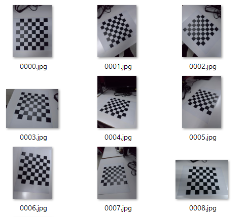
From image processing, we can obtain the 2D coordinates of the corner points in each photo.
At the same time, we know the chessboard coordinates are identical across these photos, so we can assume the chessboard 3D coordinates are $(0, 0, 0)$, $(0, 1, 0)$, $(1, 1, 0)$, $(1, 2, 0)$, $(2, 1, 0)$, … .
Then we can solve for $\mathbf H$:
$$\mathbf{\tilde m} = \mathbf H \mathbf {\tilde M}$$
One method to solve $\mathbf H$ is described in Appendix A of Zhang’s paper. We solve:
$$
\begin{bmatrix}
{\mathbf {\tilde M}}^T & \mathbf 0^T & -u {\mathbf {\tilde M}}^T\\
\mathbf 0^T & {\mathbf{\tilde M}}^T &-v{\mathbf {\tilde M}}^T
\end{bmatrix} \mathbf x = \mathbf L \mathbf x = 0
$$
Define the matrix on the left as $\mathbf L$. Expanded, it looks like:
$$
\begin{bmatrix}
&X_1 &Y_1 &1 &0 &0 &0 &-uX_1 &-uY_1 &-u \\
&0 &0 &0 &X_1 &Y_1 &1 &-vX_1 &-vY_1 &-v
\end{bmatrix}
$$
One image provides two rows. If we have $n$ images, then $\mathbf L$ is a $2n \times 9$ matrix.
The solution $\mathbf x$ is the eigenvector of $\mathbf L^T \mathbf L$ associated with the smallest eigenvalue. In code, it may be more intuitive:
L # 2n x 9 的 numpy 矩陣
w, v, vh = np.linalg.svd(L)
x = vh[-1]
The $\mathbf H$ computed from $\mathbf x$ needs to be scaled by a coefficient $\rho$:
$$
\mathbf H = \rho x = \rho
\begin{bmatrix}
x_1 &x_2 &x_3 \\
x_4 &x_4 &x_5 \\
x_6 &x_7 &x_8
\end{bmatrix}
$$
According to:
$$\mathbf{\tilde m} = \rho \mathbf x \mathbf {\tilde M}$$
My approach is to plug each corresponding coordinate pair into the equation to obtain $\rho$, then take the average.
¶ 3. Constraints on Intrisic Parameters
Define $\mathbf H = [\mathbf h_1 \quad \mathbf h_2 \quad \mathbf h3]$:
$$[\mathbf h_1 \quad \mathbf h_2 \quad \mathbf h3] = \lambda \mathbf A [\mathbf r_1 \quad \mathbf r_2 \quad \mathbf t]$$
$\lambda$ is an arbitrary coefficient. Since $r_1$ and $r_2$ are orthonormal, we have:
$$
\begin{align}
{\mathbf h_1}^T {\mathbf A}^{-T} \mathbf A^{-1} \mathbf h_2 &= 0 \\
{\mathbf h_1}^T {\mathbf A}^{-T} \mathbf A^{-1} \mathbf h_1 &= \mathbf {h_2}^T \mathbf A^{-T} \mathbf A^{-1} \mathbf h_2
\end{align}
$$
¶ 4. Solving for the Intrisic Parameters
Because the intrinsic matrix is a camera’s internal parameter, it is the same for every photo. In what follows, I skip the proof and focus directly on how to solve for the intrinsic matrix.
From Section 2, we can obtain $\mathbf H$ for each image. Then define:
$$
\mathbf B = {\mathbf A}^{-T} {\mathbf A}^{-1} =
\begin{bmatrix}
B_{11} &B_{12} &B_{13} \\
B_{12} &B_{22} &B_{23} \\
B_{13} &B_{23} &B_{33}
\end{bmatrix}
$$
$\mathbf B$ is a symmetric matrix. Define $\mathbf b = [B_{11}, B_{12} ,B_{22}, B_{23}, B_{33}, B_{11}]^T$
$\mathbf H$ is known. Let $\mathbf h_i$ denote the i-th column of $\mathbf H$, so $\mathbf h_i = [h_{i1}, h_{i2} ,h_{i3}]^T$.
Then define:
$$
\mathbf v_{ij} = [h_{i1} h_{j1}, h_{i1} h_{j2} + h_{i2} h_{j1}, h_{i2} h_{j2},
h_{i3} h_{j1} + h_{i1} h_{j3}, h_{i3} h_{j2} + h_{i2} h_{j3}, h_{i3} h_{j3}]^T
$$
Then we solve:
$$
\begin{bmatrix}
\mathbf v_{12}^T \\
{( \mathbf v_{11} - \mathbf v_{22})}^T
\end{bmatrix} \mathbf b = \mathbf V \mathbf b = 0
$$
Where $\mathbf V$ is a $2n \times 6$ matrix. One image yields two equations. With at least three planes ($n >= 3$), we can solve for $\mathbf b$.
The solution is again the eigenvector of $\mathbf L^T \mathbf L$ associated with the smallest eigenvalue:
w, v, vh = np.linalg.svd(V)
b = vh[-1]
Then we can recover the parameters from $\mathbf B$:
$$
\begin{align}
v_0 &= (B_{12} B_{13} − B_{11} B_{23})/(B_{11} B_{22} − B_{12}^2)\\
λ &= B_{33} − [B_{13}^2 + v_0(B_{12}B_{13} − B_{11}B_{23})]/B_{11}\\
α &=\sqrt{λ/B_{11}}\\
β &=\sqrt{λB_{11}/(B_{11}B_{22} − B^2_{12})}\\
γ &= −B_{12} α^2 β/λ\\
u_0 &= γv_0/β − B_{13}α^2/λ\\
\end{align}
$$
Then we obtain the intrinsic matrix $\mathbf A$. Substitute back according to the definition:
$$
\mathbf A =
\begin{bmatrix}
α &γ &u_0 \\
0 &β &v_0 \\
0 &0 &1
\end{bmatrix}
$$
¶ 5. Solving for the Extrinsic Parameters
Because $\mathbf A$ is fixed, and each image provides a homography $\mathbf H$, we can solve the extrinsic parameters.
$$
\mathbf H = [\mathbf h_1 \quad \mathbf h_2 \quad \mathbf h_3]
= \mathbf A [\mathbf r_1 \quad \mathbf r_2 \quad \mathbf r_3 \quad \mathbf t]
$$
The relationships are:
$$
\begin{align}
\mathbf r_1 &= \lambda \mathbf A^{-1} \mathbf h_1 \\
\mathbf r_2 &= \lambda \mathbf A^{-1} \mathbf h_2 \\
\mathbf r_3 &= \mathbf r_1 \times \mathbf r_2 \\
\mathbf t &= \lambda \mathbf A^{-1} \mathbf h_3 \\
\end{align}
$$
Where $\lambda$ is a scale factor (different from the previous $\lambda$), and $ λ = 1/ \Vert \mathbf A^{−1} \mathbf h_1 \Vert = 1/ \Vert \mathbf A^{−1} \mathbf h_2 \Vert$.
At this point, we have obtained both intrinsic parameters and extrinsic parameters.
¶ OpenCV calibrateCamera
With the algorithm above, we can implement a function equivalent to cv2.calibrateCamera. For comparison, here is the OpenCV cv2.calibrateCamera signature:
ret, mtx, dist, rvecs, tvecs = cv2.calibrateCamera(objpoints, imgpoints, img_size,None,None)
You can see that cv2.calibrateCamera represents extrinsics using a rotation vector and a translation vector, while we derived matrices above, so we need a conversion.
Here, rvecs contains the rotation vectors for all images, and tvecs contains the translation vectors for all images. For each image, the rotation and translation are computed as follows:
from scipy.spatial.transform import Rotation as R

# A, h1, h2, h3 為已求得 numpy 矩陣

lambda_ = 1/np.linalg.norm(np.dot(np.linalg.inv(A), h1))

r1 = lambda_*np.dot(np.linalg.inv(A), h1)
r2 = lambda_*np.dot(np.linalg.inv(A), h2)
r3 = np.cross(r1, r2
r_matrix = np.array([r1, r2, r3)]).T

t = lambda_*np.dot(np.linalg.inv(A), h3)
r = R.from_matrix(r_matrix).as_rotvec()

rvecs.append(r)
tvecs.append(t)
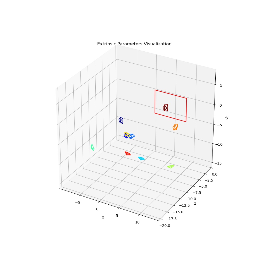
¶ Visualizing Extrinsics
After computing the extrinsics matrices, we can visualize them and recover the camera position and orientation for each photo. The small pyramid represents the camera, and the red box represents the chessboard.
¶ A Few Practical Tips
If the photos contain a chessboard, you can call cv2.findChessboardCorners directly.
You can downscale the chessboard images first: finding the pattern corners takes time, and with smaller image coordinates, the expanded matrices also become smaller.
When solving with SVD, pay attention to whether the matrix rank is sufficient to solve the system.